Our 2026 FIFA World Cup forecasts come from a statistical prediction model that blends three approaches — an Elo rating system, a Dixon-Coles Poisson goals model, and a hierarchical Poisson model — into a calibrated ensemble, then runs 100,000 Monte Carlo simulations of the tournament to estimate how often each team lifts the trophy, reaches the final, survives the group, and everything in between. This page is the full, transparent record of how those probabilities are produced — the models, the inputs, and the known limitations.
People often look for an "AI World Cup prediction." Strictly, this is a set of statistical and machine-learning models — maximum-likelihood-fit goals models, a hierarchical Bayesian layer, and an Elo rating — rather than a single neural network. The principle is the same: every number is computed from data, not hand-picked by a pundit.
We publish probabilities, not opinions and not recommendations. The numbers update when the underlying data does — new results, rating refreshes, squad changes — and the rest of this document is the complete technical record of how they are produced.
What we publish
For each of the 48 teams in the 2026 tournament, the site publishes:
P(advance from group)— probability of finishing in a qualifying position from the group stage.P(reach round-of-32),P(reach round-of-16),P(reach quarter-final),P(reach semi-final),P(reach final).P(win the tournament).
Per-fixture 1X2 (home / draw / away) probabilities are produced internally and may be surfaced on the public site once the tournament starts.
The numbers are model output, not opinion. They update only when the inputs do (rating refresh, results from any matches still being played, structural fixture changes).
How accurate is the model?
The full evaluation lives under "Walk-forward results" further down this page. The headline numbers, in plain English:
- Calibration on the tournament tier — 4.4 percentage-point expected calibration error. When the model says "35% probability", the observed frequency across matches in that band lands within roughly 4 points either side. This is the tier that publishes for WC2026; it has been validated against the same 24 months of continental-tournament and World Cup matches the calibrator was fit on (five-fold cross-validated, n = 453). The pre-calibration baseline was 7.75pp, so the per-tier calibrator buys a 44% reduction on the slice that matters.
- Brier score across two years of walk-forward backtest — 0.503 for the ensemble. Lower is better; range is
[0, 2]. For comparison: a uniform1/3, 1/3, 1/3guess scores 0.667, a frequency-baseline scores ~0.61, and a published random-forest baseline on FIFA-rating features (Tsokos et al. 2019) scores ~0.46. The ensemble matches the Dixon-Coles component on Brier and beats it on log-loss; no single component dominates. This walk-forward number is dominated by friendlies and qualifiers, and it composes the ensemble from the current Elo snapshot rather than each team's contemporaneous rating — a mild backward leak that flatters recent-window scores. - Honest, leakage-free tournament Brier — 0.572 (ECE 5.6pp). The number above is the all-competition figure. For the matches that actually matter — major tournaments — we reconstruct the full model as it stood the day before each of the 24 major-tournament editions from 2014–2024 (Dixon-Coles + Hierarchical Poisson refit on prior matches, Elo rolled forward match-by-match, calibrator refit on only the preceding 24 months) and score all 987 matches with zero look-ahead in any layer. That leakage-free out-of-sample Brier is 0.572 with a 5.6pp expected calibration error — the canonical expectation for WC 2026. The per-tournament breakdown and reliability diagrams are on the calibration scoreboard; single-fold tournament-slice estimates (~0.545) read lower because they carry the same snapshot leak.
- Eight non-overlapping 90-day evaluation windows, 2,033 international matches total. The walk-forward refits every fold on data strictly before that fold's evaluation start, so there is no look-ahead bias. The harness lives in
scripts/backtest_models.pyand runs end-to-end in a few minutes on a laptop.
What this does not tell you: a model that scores well on the international corpus can still miss specific tournaments (the population of tournament-relevant fixtures is small relative to the population of friendlies the fit trains on). The honest read on those numbers is "comparable to research baselines and well-calibrated on tournament-tier matches"; it is not "guaranteed predictive". See "Limitations and caveats" below for the full disclosure.
How we generate the probabilities
We run four families of model, plus a uniform-weighted ensemble across the three that produce coherent per-match 1X2 distributions. A fifth model rates individual players and feeds the per-player surfaces.
Model 1 — Per-match Elo with Monte Carlo bracket simulation
A FIFA-Elo formula maps two teams' ratings to expected score, applying a 100-point home-advantage adjustment (zeroed on neutral venues) and a fixed 22% draw probability. The full 104-fixture bracket is replayed in 100,000 Monte Carlo simulations and the per-team round-by-round probabilities are aggregated from the simulation outputs. Each per-fixture sample now consumes the calibrated ensemble's P(H/D/A) (see "Ensemble" below) rather than raw Elo, so the bracket's probability shape inherits the ensemble's calibration.
Inputs: per-team international Elo from eloratings.net, the 48-team group draw, and the published 2026 fixture list.
This is the simplest, lightest model in the stack. It does not fit anything — it consumes a published rating directly and propagates it through the bracket.
Model 2 — Dixon-Coles with time decay
Per-team attack and defence parameters fit by maximum-likelihood on roughly forty-nine thousand international results since 1872. Goals follow Poisson with rate λ = exp(home_adv + attack[home] − defence[away]). The Dixon-Coles ρ parameter corrects the joint probability of 0–0, 0–1, 1–0, and 1–1 outcomes, addressing the well-known Poisson under-fit to low-scoring draws. An exponential time-decay weight with a five-year half-life emphasises recent form (the half-life is longer than the standard 18 months used for club football because international matches are sparser per team); apart from that decay, every match contributes equally to the likelihood. We do not down-weight friendlies relative to competitive matches in this goal-rate fit: that adjustment suits an outcome-based Elo update (where friendly experimentation is noise), but a leakage-safe walk-forward backtest showed it measurably hurts the goal-rate model's accuracy on tournament fixtures, so the Dixon-Coles and Hierarchical-Poisson fits weight all matches equally.
Inputs: international match results (date, teams, scores, tournament tier) since 1872. In production the per-match Poisson response is xG where available (StatsBomb open data, 342-match single-provider corpus), falling back to realised goals — see "International xG as the response" below.
Output: per-fixture λ_home, λ_away, from which a coherent joint goal distribution — and therefore P(home/draw/away), goal-differential distributions, total-goals distributions, and exact-score grids — falls out by marginalisation.
International xG as the response
The improvements roadmap (§1.2) called out replacing realised goals with expected goals as the Poisson response as the single highest-leverage remaining accuracy lift. As of 2026-05-29 this is wired into the production fit path (the daily auto-refit fits Dixon-Coles with --use-xg and refits the ensemble calibrator on the xG-enabled ensemble; the xG-enabled artefacts regenerate on the first refit after the change lands): Dixon-Coles and the uniform Ensemble use the xG response; the hierarchical Poisson is excluded (it fails the calibration half of the gate). The full backfill + gate write-up is documentation/research-notes/intl-xg-statsbomb-backfill.md.
Data — single-provider StatsBomb open data. The legacy scripts/pull_intl_xg.py pulls Opta xG from the JaseZiv/worldfootballR_data mirror, but that mirror is stale: it carries xG for only ~143 matches (WC 2018, Euro 2020, Copa 2021), WC 2022 is present-but-null, and Euro 2024 / Copa 2024 / AFCON 2023 are absent — and FBref-live / FotMob per-match endpoints are Cloudflare/Turnstile-walled. So scripts/pull_intl_xg_statsbomb.py sources the gap from StatsBomb open data (raw.githubusercontent.com/statsbomb/open-data), computing per-match team xG as the sum of every shot's shot.statsbomb_xg. To avoid mixing provider models (Opta vs StatsBomb xG are not directly comparable — see Risk note), we went single-provider: StatsBomb open data also covers WC 2018 + Euro 2020, so those two Opta-baseline tournaments are re-derived from StatsBomb and replace the Opta rows. Coverage:
- StatsBomb (314 rows): WC 2018 (64), WC 2022 (64), Euro 2020 (51), Euro 2024 (51), Copa America 2024 (32), AFCON 2023 (52).
- Opta residual (28 rows): Copa America 2021 — StatsBomb open data does not cover it. This is the only provider heterogeneity left, tagged
source_xg_model="opta".
Total: 342 matches (data/raw/intl/xg.csv, gitignored, regenerated by the puller). Each row is snapped to the pull_intl_results orientation + date so it joins the fit corpus cleanly; 339/342 join (the 3 misses are residual Opta Copa-2021 name/orientation rows inherited from the legacy baseline).
Integer-Poisson choice. The Poisson likelihood requires non-negative integer support. xG is continuous. We discretise via round(xG) (nearest integer, banker's rounding), which preserves the existing optimiser + prediction code and is unbiased on average (E[round(X)] ≈ E[X] for continuous X with mean ≳ 1, the regime in football match xG). ceil would inflate goal rates by ~0.5/match; floor would deflate symmetrically; round is the natural unbiased choice. Provider-level xG differences of ~0.1–0.2 per shot wash out under this rounding, which is why a 314/28 single-provider-plus-residual corpus is fit-safe.
Fallback discipline. The xG/goals decision is per-match. A match with both home_xg and away_xg populated and finite uses round(xG) as the Poisson response on both sides; any match missing either side falls back to the realised goal count. The fit reports the per-fit coverage rate in xg_meta metadata on the output JSON. A 10-year DC window sees ~3.7% of training matches (339) using xG and the rest falling back to goals.
Gate outcome — cleared for DC + Ensemble. The acceptance gate (documentation/improvements-roadmap.md Spec B) is median Brier strictly lower than the uniform-goals baseline AND ECE within +0.2pp, across the 8-fold walk-forward. In production the xG response is enabled for DC only, so the gate is measured in that configuration (scripts/backtest_models.py --use-xg --xg-dc-only):
- Tournaments-only slice (k≥50, n=311): DC ΔBrier_median −0.0023 / ΔECE −0.41pp → PASS; Ensemble ΔBrier_median −0.0016 / ΔECE −1.15pp → PASS.
- Whole-corpus (n=1,930): DC ΔBrier_median −0.0004 / ΔECE +0.08pp → PASS; Ensemble ΔBrier_median −0.0006 / ΔECE −0.38pp → PASS.
Hierarchical Poisson is excluded. Under the xG response HP improves Brier but its whole-corpus ECE drifts +0.21pp, just over the +0.2pp tolerance, so production keeps HP on realised goals. The production ensemble is mean(Elo, DC-xg, HP-goals). This is fit_models_pre_cutoff(use_xg=True, use_xg_hp=False).
Production path + calibrator refit. .github/workflows/auto-refit.yml (daily) pulls StatsBomb xG, fits DC with --use-xg, leaves HP on goals, and fits the ensemble calibrator with --use-xg. The last point is load-bearing: the per-class isotonic/Platt calibrator re-fits the ensemble internally rather than reading dixon_coles.json, so enabling xG for DC shifts the distribution it must calibrate — fit_ensemble_calibrator.py --use-xg refits it on the xG-enabled ensemble (use_xg_dc: true recorded in the artefact). Verified: the xG calibrator's tournament-tier OOF ECE (10.01pp) matches the no-xG one (10.09pp) — no calibration regression. scripts/fit_dixon_coles.py --use-xg and scripts/fit_hierarchical_poisson.py --use-xg retain the per-match opt-in flag; scripts/backtest_models.py --use-xg [--xg-dc-only] runs the comparison.
Risk note. xG from different providers (Opta via FBref vs StatsBomb vs in-house club models) is not directly comparable. We are single-provider (StatsBomb) except for the 28 Copa-2021 Opta rows StatsBomb does not cover; that residual is isolated by source_xg_model and is a small minority of a corpus where rounding already absorbs sub-shot provider differences. Any future second xG source lands as a distinct source_xg_model value, handled by the same orientation-aware merge (StatsBomb-preferred) — not free mixing.
Model 3 — Hierarchical Bayesian Poisson (full posterior via PyMC NUTS)
The same likelihood as Model 2, with Gaussian priors on the per-team attack and defence parameters. The priors implement partial pooling: data-rich teams (Brazil, Germany) follow the data; sparse teams (Tuvalu, Bermuda) are shrunk toward the population mean. Estimation is by NUTS in PyMC (1,000 warmup + 1,000 sampling iterations across 4 chains, ~250 teams × 2 parameters plus home_advantage and ρ). Convergence is gated on max R-hat ≤ 1.01 and minimum effective sample size ≥ 400 across all parameters; the fit script raises rather than ships if either gate fails. A thinned posterior is written to data/wc2026/hierarchical_poisson_samples.npz (~4,000 draws after warmup) alongside the posterior-mean JSON used by the ensemble.
Inputs: identical to Model 2.
Output: identical interface to Model 2 at the point-estimate level (posterior means in place of MAP values). Additionally, every parameter carries posterior samples that propagate through the bracket Monte Carlo to produce credible intervals on each published per-team progression probability.
Model 3b — Confederation-pooled variant (two-level partial pooling)
Same likelihood and same home_advantage / ρ priors as Model 3. The change is the prior layer on the per-team attack and defence parameters: instead of pooling every team against a single global mean (attack[i] ~ Normal(0, σ_attack)), each team's prior is centred on its confederation's posterior mean with confederation-specific shrinkage:
mu_attack_confed[c]    ~ Normal(0, 0.5)
sigma_attack_confed[c] ~ HalfNormal(0.5)
attack[i] ~ Normal(mu_attack_confed[c_i], sigma_attack_confed[c_i])
and identically for defense. Confederations are the six FIFA confederations (UEFA, CONMEBOL, CAF, AFC, CONCACAF, OFC) plus an OTHER bucket for non-FIFA entities that turn up in the upstream RSSSF corpus (regional sides like Yorkshire / Padania, breakaway-region selects, microstates not affiliated with FIFA). Confederation assignments come from data/wc2026/teams.csv for the 48 qualified teams (authoritative) and a static FIFA-membership table covering the remaining ~190 nations in the fit window.
Why. The data-rich confederations (UEFA, CONMEBOL) have qualitatively different scoring patterns from the data-sparse ones (CAF, AFC, OFC) — those differences are real and persist even after controlling for individual team quality. Global-mean pooling drags Curaçao, Cape Verde, New Caledonia toward the same population mean that Germany and Brazil contribute to, which is poor regularisation for sparse-data teams. Pooling within confederation lets each region's overall scoring level inform the prior for its small members. Posterior summary of the confederation-level means at the current refit (NUTS, 4 chains × 1,500 draws after 2,000 warmup, max R-hat = 1.008, min ESS = 496, zero divergences):
| Confederation | n teams | μ_attack | μ_defence | σ_attack | σ_defence |
|---|---|---|---|---|---|
| UEFA | 55 | +0.61 | +0.58 | 0.58 | 0.42 |
| CONMEBOL | 10 | +0.90 | +0.94 | 0.31 | 0.37 |
| CAF | 54 | +0.28 | +0.31 | 0.34 | 0.40 |
| AFC | 47 | -0.15 | -0.21 | 0.66 | 0.71 |
| CONCACAF | 41 | -0.24 | -0.44 | 0.61 | 0.67 |
| OFC | 12 | -0.79 | -0.99 | 0.71 | 0.91 |
| OTHER | 25 | -0.20 | -0.64 | 0.32 | 0.55 |
The ordering matches a priori expectations — CONMEBOL and UEFA on top, OFC at the bottom — and σ is widest in AFC / CONCACAF / OFC, where the within-confederation spread of team quality is genuinely larger than in UEFA / CONMEBOL.
OTHER-bucket coverage gap. 25 teams land in OTHER after the confederation lookup completes — almost entirely non-FIFA regional sides (Abkhazia, Padania, Yorkshire, Sápmi, Tibet, regional Norwegian island sides). These teams' priors pool against each other, which is the honest default: we genuinely have no continent-level mean to pool them toward. The bucket is large enough to identify its own μ and σ without dominating any FIFA confederation's posterior.
Acceptance gate. The walk-forward backtest harness (scripts/backtest_models.py --with-confed-hp) refits both the global-pool and confed-pool HP MAP variants at each fold's cutoff and compares Brier scores on the post-cutoff eval window, both overall and on a sparse-data team subset (FIFA rank ≥ 60 or non-WC). A faster single-fold complement (scripts/backtest_confed_hp_gate.py) writes data/wc2026/confed_hp_gate.json for cases where the 8-fold runtime is prohibitive.
On the most recent single-fold gate (fit cutoff 2025-05-22, 365-day eval window, n = 949 common predictions):
| Subset | Global-mean HP Brier | Confed-pool HP Brier | Δ |
|---|---|---|---|
| Overall (all matches) | 0.4869 | 0.4845 | -0.0024 |
| Sparse-data team subset (FIFA ≥60 OR non-WC), n = 877 | 0.4722 | 0.4699 | -0.0022 |
The confed-pool variant is strictly better on both subsets. The lift is in the predicted direction (the §16 spec forecast 0.5–1pp on sparse teams; we observe ~0.2pp on average across the eval window) and clears the gate's "median Brier strictly lower on sparse-data teams" criterion. Where the lift concentrates is informative — the per-confederation breakdown on the same gate:
| Confederation (matches with ≥1 team in it) | n | Global Brier | Confed-pool Brier | Δ |
|---|---|---|---|---|
| OFC | 23 | 0.627 | 0.495 | -0.132 |
| AFC | 213 | 0.509 | 0.499 | -0.010 |
| CONCACAF | 214 | 0.514 | 0.505 | -0.009 |
| UEFA | 301 | 0.464 | 0.461 | -0.003 |
| CONMEBOL | 76 | 0.541 | 0.545 | +0.004 |
| CAF | 312 | 0.499 | 0.504 | +0.005 |
| OTHER | 8 | 0.532 | 0.566 | +0.035 |
OFC delivers nearly all of the lift — the within-confederation prior is dramatically more informative for the dozen Oceania nations than the global-mean prior was. AFC and CONCACAF also improve. CAF, CONMEBOL, and the small OTHER bucket regress slightly, but the regressions are small (< 0.01) and on smaller-n subsets where one fewer correct prediction would close the gap. The aggregate is net positive on the sparse subset, which is the gate that matters.
Top WC-team net-rating shifts under confederation pooling. The largest shifts land in the small confederations the change was designed to help — New Zealand drops 0.25 in net (attack − defence) under OFC-pooling vs the global mean; Canada and Japan each shift 0.05–0.06 toward the AFC / CONCACAF lower confederation means. These are the teams whose downstream tournament probabilities move most when the confed-pooled posterior replaces the global-pool one.
Output: the confed-pooled fit writes the same data/wc2026/hierarchical_poisson_samples.npz posterior schema as the global-pool fit (the (S, T, 2) team_attack_defense array plus home_advantage, rho, team_ids), so the bracket Monte Carlo's posterior-uncertainty path consumes it without changes. Additive arrays carry the confederation-level hyper-posterior samples for the per-confederation surfaces.
Ensemble — uniform average of Models 1, 2, and 3 with per-tier isotonic calibration
For each fixture we compute P(H/D/A) under each of the three component models and take the uniform mean. If a component cannot predict a fixture (Elo, for instance, has no rating for a non-WC team), it is dropped and the mean is taken over the remaining components. The ensemble's per-component breakdown is kept alongside its averaged output so the contribution of each is traceable.
On top of the uniform average we apply a per-class isotonic calibrator. The calibrator is fit by pool-adjacent-violators (a non-parametric monotone regression) against held-out match outcomes — one curve per outcome class (home / draw / away) — then renormalised so the three calibrated probabilities sum to one. The artefact (data/wc2026/ensemble_calibrator.json) carries three sets of curves keyed by tournament tier — friendly, qualifier, and tournament (which pools continental finals and the FIFA World Cup itself) — plus a pooled-across-tiers set retained for backwards compatibility. At predict time we look up the tier from the fixture's tournament and apply the matching curves. Pooling friendlies and qualifiers with major tournaments dilutes the calibration on the slice that matters for WC publication; splitting by tier is cheap and resolves it.
The tournament tier uses a hybrid calibrator window: 24 months of tournament-tier matches augment the standard 12-month holdout. At 12 months only ~70 tournament matches are available — too few for isotonic PAV, which collapses to the identity (y=x) curve. At 24 months n=453 and PAV fits stably. Friendlies and qualifiers keep the 12-month window where n is already sufficient.
The artefact also carries per-tier Platt temperature scaling parameters (T per tier, where p_cal ∝ p_raw^(1/T) then renormalise). Temperature scaling fits stably at low n and serves as a fallback when isotonic collapses. In practice, isotonic wins for tournament tier (4.39pp vs 6.99pp) and Platt wins for qualifiers (5.07pp vs 5.59pp pooled isotonic). The best_for_tournament field on the artefact records which variant the cross-validation selected for the tournament slice.
Five-fold cross-validated ECE on the holdout (n = 1,319 common-subset matches after hybrid augmentation), per tier:
| Tier | n | Uncalibrated | Pooled isotonic | Tier isotonic | Tier Platt |
|---|---|---|---|---|---|
| friendly | 409 | — | — | — | 5.59pp |
| qualifier | 457 | — | — | — | 5.07pp |
| tournament (continental + WC) | 453 | 7.75pp | 6.31pp | 4.39pp | 6.99pp |
The acceptance gate is tournament-tier CV ECE strictly lower under tier-aware — the slice that publishes for WC2026. The gate passes (7.75pp uncalibrated → 4.39pp tier-isotonic, a 44% reduction). The bracket-MC sampler consumes the same artefact, with a refinement: group-stage simulations use the raw (uncalibrated) ensemble probabilities because the tournament-tier calibrator pools group and knockout matches and consequently suppresses draws (~26% empirical → ~16% calibrated). Knockout-stage simulations keep the fully calibrated probabilities.
Extremization removed (2026-06-10). The Ranjan-Gneiting (2010) extremization step (d = 1.15) has been disabled (d = 1.0, i.e. no-op) after a walk-forward sweep over d in {1.00, 1.05, ..., 1.30} showed a monotonic worsening as d increases: d=1.0 Brier 0.49866 vs d=1.15 Brier 0.50134, a 26.8bp gain from disabling it. The theoretical premise (that linear pools of calibrated forecasters are underconfident) does not hold when one component (Elo, with its fixed 22% draw rate) is itself poorly calibrated; extremizing amplifies the miscalibration rather than correcting underconfidence. See postprocess-tuning-sweep research note.
Group-stage draw scaling. Group-stage simulations apply a small constant multiplicative scaling GROUP_STAGE_DRAW_FACTOR = 1.05 to the raw draw probability before renormalisation: P(draw) <- 1.05 * P(draw_raw), then divide each of P(H/D/A) by the new sum. The Brier response is a plateau across roughly 0.99-1.07, so the exact factor barely matters; 1.05 is the sweep minimum over 692 group-stage matches (all World Cups). The factor applies to group-stage bracket sampling only. A per-matchday refinement (separate factors for matchday 1 vs matchday 3 dead-rubber slates) was tested and rejected: the bootstrap CI on the Brier delta did not exclude zero, so the flat factor is what ships (hidden-motivations research note for the full backtest).
The uniform-weighted blend is the simplest possible combination of the three component models and is what production currently uses. Two learned alternatives have been backtested against it: a Bayesian stacking-weights variant (see "Bayesian stacking weights" below) that learns three weights (w_elo, w_dc, w_hp) on the 3-simplex, and a richer gradient-boosted meta-learner (see "Stacked meta-learner" below) that consumes the three component probabilities plus ~20 per-fixture covariates. Both are shipped as code + walk-forward infrastructure + fitted artefacts; both are tested under the same median-Brier-strictly-lower-than-uniform gate that the improvements roadmap documents. The production predict path keeps the uniform mean + isotonic calibrator until one of the learned variants clears that gate.
Bayesian stacking weights on the three components — §1.5
A simpler learned ensemble than the gradient-boosted meta-learner: pick three weights w = (w_elo, w_dc, w_hp) on the 3-simplex (w_k ≥ 0, Σ w_k = 1) that maximise the held-out log-score
L(w) = Σ_i log(Σ_k w_k · p_k(y_i | x_i))
over walk-forward observations. This is the Yao et al. 2018 stacking objective ("Using stacking to average Bayesian predictive distributions", arXiv:1704.02030), with walk-forward leave-one-out as the honest backtest discipline instead of Pareto-smoothed importance sampling (refitting the component models per walk is what we already do; the implementation reuses backtest_models.fit_models_pre_cutoff). The simpler objective trades the meta-learner's ~20-feature surface for three free parameters — the right capacity envelope when the meta-learner is on the overfitting edge at n ≈ 2k.
Optimisation: scipy.optimize.minimize with method=SLSQP, sum-to-one equality constraint, [0, 1] box bounds on each component, and an analytic gradient (scripts/fit_stacking_weights.py). Starting point is the uniform centroid (1/3, 1/3, 1/3).
The walk-forward harness is the same as the meta-learner's: at each walk, weights are fit on the accumulated rows from EVERY earlier walk and evaluated on this walk. The first walk has no training pool and reports the uniform baseline. The shipped artefact (data/wc2026/stacking_weights.json) carries the union-of-walks weights and the per-walk + aggregate metrics so the gate decision is auditable.
Status — negative result. The walk-forward fit produced learned weights w = (w_elo = 0.316, w_dc = 0.627, w_hp = 0.056) over n = 2,074 accumulated training rows. Aggregate metrics across the eight walks (see "Walk-forward results" for the complete per-fold table):
| Variant | Brier (mean) | Brier (median) | log-loss (mean) | ECE (mean) |
|---|---|---|---|---|
| Uniform-average ensemble | 0.5062 | 0.4941 | 0.8582 | 7.40pp |
| Bayesian stacking weights | 0.5062 | 0.4954 | 0.8581 | 7.47pp |
The stacking-weights ensemble ties on Brier mean and log-loss mean to four decimal places, and loses on median Brier by 0.0013 (the acceptance gate is strictly lower median Brier than the uniform baseline). The artefact ships, but the production predict path stays on the uniform mean + isotonic calibrator. predict_stacked is wired in as an opt-in by passing use_stacking=True through ensemble.load_components and substituting predict_stacked for predict_match.
The result is informative: the optimiser concentrates 94% of the weight on Elo + Dixon-Coles and almost discards Hierarchical Poisson (w_hp ≈ 0.06) — a signal that under the LOO log-score on this dataset HP's contribution is largely captured by DC, which it shares the goal-process likelihood with. The per-walk weights are not stable across walks (the Elo weight ranges 0.24 → 0.51 across walks where a fit was possible), which suggests the simplex objective is finding a flat optimum and the three components really do have correlated errors at this n. Compare to the §1.1 gradient-boosted meta-learner from PR #274, which lost on median Brier by ~30pp (0.5339 vs 0.4977) — the stacking-weights approach is much closer to uniform but still doesn't clear the gate.
Predict-side: scripts/ensemble.predict_stacked consumes the artefact and computes p = w_elo · p_elo + w_dc · p_dc + w_hp · p_hp per fixture, then applies the same per-class isotonic calibrator as the uniform path. Falls back to predict_match (uniform mean) when the artefact is missing.
Stacked meta-learner over the three components plus per-fixture covariates
A regularised gradient-boosted classifier (sklearn.ensemble.HistGradientBoostingClassifier, max_depth=4, learning_rate=0.05, L2 regularisation, early stopping on a 10% internal validation hold) consumes the three component models' per-fixture P(H/D/A) plus a small set of per-fixture covariates:
- Neutral-venue flag.
- Tournament tier (one-hot: friendly / qualifier / continental / World Cup).
- Days since each side's last international match.
- Confederation pair (label-encoded).
- Per-venue altitude, mean temperature, and mean precipitation (from the per-venue climatology snapshot).
The target is the observed 1X2 outcome; the objective is multinomial log-loss. The fit is walk-forward (see "Walk-forward evaluation" below): each walk's training rows are the pooled feature rows from every earlier walk's evaluation window, so no walk's metrics use any data from its own evaluation rows. A per-class isotonic calibrator is fit on top of the meta-learner's predictions (same pool-adjacent-violators procedure as the uniform-ensemble calibrator) so the meta path keeps the same calibration discipline.
Status — negative result. The walk-forward backtest harness, the meta-learner fitting code (scripts/fit_ensemble_meta.py), and the production-side predict_meta path (with isotonic post-calibrator and uniform-mean fallback) are all shipped. The fitted artefact (data/wc2026/ensemble_meta.json) was produced on the live data — and on the 8-fold walk-forward evaluation it does not beat the uniform-average ensemble.
Aggregate metrics across all 8 walks (see "Walk-forward results" for the complete per-fold table):
| Variant | Brier (mean) | Brier (median) | log-loss (mean) | ECE (weighted) |
|---|---|---|---|---|
| Uniform-average ensemble | 0.503 | 0.498 | 0.855 | 6.1pp |
| Stacked meta-learner | 0.533 | 0.534 | 1.029 | 7.5pp |
The meta-learner loses on the median Brier across walks (the acceptance gate documented in documentation/improvements-roadmap.md Spec B), and loses on every individual walk that supplied training data. The shipping ensemble remains the uniform-average + isotonic calibrator path.
Why the lift didn't materialise. With ~1,900 accumulated rows by the final walk and ~20 features, an HistGradientBoostingClassifier with max_depth=4 is on the overfitting edge for a small-effect-size 1X2 problem. Groll's hybrid random-forest lineage reports 1–3pp Brier gain over a single-component baseline, but those papers train on a tournament-specific dataset (a few hundred matches) with external-rating features we do not use and evaluate over a single tournament — a different regime from international-football walk-forward. The honest signal from this experiment is that on n ≈ 2k and uncorrelated component errors that are already small, the gradient-boosting recipe needs more data, stronger feature engineering, or a simpler stacking objective (per documentation/improvements-roadmap.md §1.5 Bayesian stacking weights) to beat the uniform mean.
The meta-learner artefact + walk-forward harness are kept on the branch: when the training pool grows (after another tournament cycle the pool roughly doubles), the same comparison can be rerun cheaply. scripts/ensemble.py:predict_meta is already wired; switching production over is a single artefact regenerate + a flag flip in the export pipeline once the median-Brier gate is cleared.
Model 4 — Player composite rating
For surfaces that rank individual players, we compute a per-player composite in [0, 1] combining position-relevant per-90 statistics from FBref with log Transfermarkt transfer valuation as a shrinkage prior. Weights are position-specific (forwards lean on npxG and xAG; full-backs lean on progressive carries and defensive actions; centre-backs lean on aerial and tackling actions). The composite is percentile-ranked within position so the resulting rating is comparable across teams.
This rating drives the per-player surfaces only; it does not currently feed back into the team-level models.
Model 4b — Goalkeeper-specific rating
The standard composite (Model 4) is position-agnostic and its FW / MF-shaped per-90 features are meaningless for goalkeepers; for GK rows it falls back to TM-only, which over-weights backup keepers at big clubs. Model 4b produces a separate shot-stopping rating, using whichever signal is strongest for each keeper.
The signal sources are tiered:
- PSxG+/- per 90. The headline shot-stopping metric — post-shot expected goals minus goals allowed — averaged over the last three complete Big-5 seasons (2019-20, 2020-21, 2021-22) in the JaseZiv advanced-keepers parquet. 2022-23 is excluded because the mirror was archived 2025-09-18 with that season only partly populated. Raw PSxG+/- per 90 is blended 60/40 with a log-intl-caps percentile so a keeper's national-team first-choice status influences the rating; pure PSxG would under-rate first-choice international keepers whose club PSxG is unspectacular.
- Save percentage. Minutes-weighted save_pct across the same three seasons in the basic keepers table, for keepers with basic but not advanced data. Same 60/40 blend with log-caps.
- Caps + TM fallback. For keepers with no Big-5 keepers data at all — most non-Big-5 first-choice keepers and national-team backups. Blends international caps (heavily) with TM market value.
Each cohort's percentile is mapped onto a tiered [0, 1] band — psxg → [0.60, 1.00], save_pct → [0.40, 0.65], caps_tm_fallback → [0.00, 0.55] — so source quality drives the score floor. The bands overlap deliberately at the boundaries so a poor-PSxG Big-5 keeper can drop below a top save_pct keeper, and a top fallback keeper can sit close to the save_pct band (capturing players like Diogo Costa whose only Big-5 footprint is brief).
Output: data/wc2026/gk_rating.csv. The rating addresses the v0 issue that the position-agnostic composite mis-ranked keepers; not yet fed back into the team-level models.
Model 5 — Tournament-scorer probability
For each player on a 2026 WC squad, we publish the model's estimate of P(player scores ≥1 goal across the tournament). The decomposition is multiplicative: λ_match = npxG_per_90 × E[minutes]/90 × team_xG_share × opp_def_factor, then P(score ≥1 in one match) = 1 − exp(−λ_match), and finally P(score ≥1 in the tournament) ≈ 1 − (1 − P_per_match)^E[matches]. Inputs: each player's most recent ≥500-minute Big-5 npxG/90, an expected-minutes estimate from a two-state starter/substitute mixture, a position-weighted share of team xG (FW 4× / MF 2× / DF 1× / GK 0 normalised within a 4-3-3), an opponent-defence multiplier from the team-average xG-against across the other 47 WC nations, and the team's expected number of WC matches from Model 1's bracket Monte Carlo. The output drives the /scorers/ surface. v0 simplifications: no penalty-taker designation, no set-piece-taker bonus, no rotation, constant within-position xG share. A stage-conditional refinement updates per-stage P(scores ≥1) so the output reflects the conditional structure of the tournament rather than a flat per-match probability.
§2.5 update (2026-05-24). The npxG_per_90 input is now an explicit two-factor decomposition with position-prior shrinkage on the per-shot factor: npxG_per_90 = shots_per_90 × shrink(npxG_per_shot, total_shots, position), where shrink(Q, N, pos) = (N·Q + 20·μ_pos) / (N + 20) pulls per-shot toward a shots-weighted position prior (FW 0.138, MF 0.108, DF 0.087, GK 0.069). This replaces the legacy single per-90 aggregate for the 624 / 2,586 players whose source row carries shots data (the rest still go through the legacy path or position fallback). The change is surface-only — no ensemble gate applies because Model 5 doesn't feed the headline match ensemble — but the per-player popover on /scorers/ now surfaces shots/90 and observed-vs-shrunk npxG/shot so a reader can see which combination of volume and quality drives each player's headline. Source tag stats_xs_xg on anytime_scorer.csv flags the decomposition path. See scorer-xs-xg-decomposition for hypothesis, top-10 reordering, and shrinkage hyperparameter rationale.
§2.5 per-fixture opp rescaling (2026-05-26). The per-fixture top-3 scorers shown on /fixtures/<id>/ used to display P(scores in this match) computed against the team's rolling cross-WC average opponent (the opp_def_factor_avg column on anytime_scorer.csv). The figure is now rescaled to the actual fixture opponent: λ_base = npxG_per_90 × E[minutes]/90 × team_xg_share is recovered from the row, multiplied by the opponent's defence factor from intl_xg_against.csv (centred at 1.0 across the 48 WC teams), and P(scores) = 1 − exp(−λ_base × opp_def_factor[opponent]). Forwards facing a leaky defence show a materially higher per-match figure on the fixture page than facing a tight one; the tournament-level number (p_score_tournament) is unchanged because it already chains per-stage opp factors. Top-N membership is invariant under the rescaling — the opp factor is a positive multiplicative constant on all of a team's players, so within-team ordering is preserved. Falls back to the cross-WC average when the opponent is absent from the factor map (coverage gaps in intl_xg_against.csv, ~12 of 48 teams).
Predicted-XI start_prob layer (2026-05-27). The start_prob input that drives E[minutes] now has an optional third layer above the existing timeline → caps fallback chain: Model #4's predicted_squads.json is consulted first for each (team, player) pair, with the player's starting-XI / bench classification mapped to a probability band (0.85 / 0.10 for "predicted" status teams, 0.75 / 0.15 for "wikipedia_pool"). The layer is opt-in via --start-prob-source predicted_xi; the default remains timeline (legacy chain). A new start_prob_source column on anytime_scorer.csv records which layer fired per player. The proxy backtest in anytime-scorer-startprob-v2 found no Brier lift over the caps signal on a 2025 "scored any intl goal" outcome — but the backtest is contaminated (today's predicted-XI is built post-2025) and the available outcome is goal-rate-dominated rather than minutes-dominated, so the negative result is treated as inconclusive. The flag will flip default-on once an uncontaminated historical predicted-XI snapshot is available.
Model 14 — Set-piece-aware Dixon-Coles (experimental, not in production)
An attempt to extend Model 2 with a per-team set-piece-propensity lift parameter, regularised toward the team's centred set-piece-share feature from set_piece_xg_share.csv. Prior strength scales with the volume of player-season data available; teams with no row in the CSV are held at lift=0 by a very strong prior.
The fit produces data/wc2026/dixon_coles_set_piece.json. The comparative backtest applied a ship/no-ship gate (Brier strictly lower AND ECE within +0.2pp of baseline DC).
Re-evaluation on the 2026-05-22 walk-forward harness (8 folds × 90 days, n=2,033 holdout matches across 2024-06 → 2026-05): Model 14 v0 does not clear the gate. Baseline DC: weighted-mean Brier 0.5041, ECE 6.0pp. Set-piece-aware DC: Brier 0.5120 (+0.0079 worse), ECE 5.6pp (-0.4pp better). The ECE improvement is within slack but the Brier degrades, so the conjunction fails. Per-walk Brier moves: 6 of 8 walks have SP-aware ≥ baseline, with one walk (2026-02-21 → 2026-05-22) +0.047 worse. The largest per-team lifts the model fits — Canada (+0.188), Tunisia (+0.136), Ecuador (+0.113) — translate into large P(home win) swings on synthetic neutral-opponent matchups (New Zealand +22pp, Canada +17pp, USA +17pp) but those swings do not improve out-of-sample 1X2 calibration. The model is preserved on disk and the flag remains opt-in (scripts/fit_dixon_coles.py --set-piece-aware) for a v1 attempt that conditions on the fixture-conditional taker identity now available in set_piece_takers.csv.
Model 16 — Player-aware composite-differential offset (lineup-aware DC/HP extension)
A per-fixture log-rate offset that lets the projected starting-XI quality differential between two sides shift the Dixon-Coles and Hierarchical-Poisson predictions. For each WC2026 team we sum the Model-4 composite ratings of the eleven players in its projected XI (read from web/public/predicted_squads.json, the in_probable_xi=True rows). The per-team total lives in data/wc2026/team_composite_sum.csv; teams with partial XI coverage have their total normalised upward as mean_composite × 11 so under-coverage doesn't systematically depress a team. On the 2026-05-23 build all 48 squads resolve a full XI in the composite, so no team is normalised in shipping output.
The offset is additive in log-rate units:
Δ = α × (composite[home] − composite[away])
λ_home  ← λ_home  × exp(+Δ)
λ_away  ← λ_away  × exp(−Δ)
The coefficient α is calibrated by walk-forward grid search (scripts/backtest_composite_offset.py) over {0.0, 0.005, 0.01, 0.02, 0.05}. Ship gate: median Brier across the same eight 90-day walks used elsewhere must be strictly below the no-offset baseline. Gate cleared at α = 0.05 — median Brier 0.49963 vs 0.50192 baseline on the DC + HP uniform-mean row (8-fold, 2026-05-25 refit after the cross-league composite). The response is monotone across the grid (Δ Brier of −0.3 bp at α=0.005 → −2.29 bp at α=0.05), confirming the inflection sits at or above the upper edge of the grid.
α = 0.05 sits at the upper edge of the v0 grid; that the response is monotone across the grid suggests a slightly larger α might extract another fraction of a Brier point. We do not chase that in v0 — the spec set the grid and a five-point grid on noisy 8-fold medians is the calibrated answer it produces. Re-tuning α is a follow-up once the next tournament cycle expands the walk-forward pool. The calibrated coefficient is stamped into dixon_coles.json and hierarchical_poisson.json via scripts/apply_composite_alpha.py; the ensemble path reads it automatically. The default-off path (α = 0) reproduces the pre-offset ensemble bit-for-bit, so the change is reversible by re-running apply_composite_alpha.py --alpha 0.0. (Superseded — see the 2026-06-07 status update below. The apply step was never wired into the auto-refit chain, so the offset in fact shipped OFF for weeks; on re-evaluation the lift collapsed into noise and a placebo permutation test could not distinguish it from random team↔composite shuffles, so Model 16 is RETIRED as a no-ship. The offset is OFF; the shipped model is the plain Elo/DC/HP ensemble.)
Cross-league composite refresh (2026-05-25). The composite ratings the offset consumes were re-derived after PR adding scripts/build_player_composite.py's ClubElo league strength multiplier (see documentation/research-notes/cross-league-strength-factor.md). The α-grid was re-run against the new composite — α = 0.05 still wins, with the gate clearance widening from ~2.2 bp to 2.29 bp. No apply_composite_alpha action needed; the calibrated α is unchanged.
Status update (2026-06-07) — re-wired, briefly shipped at α = 0.01, then RETIRED as a placebo no-ship. The sequence:
-
The offset was silently disabled in production.
apply_composite_alpha.pystampscomposite_alphainto the DC/HP JSONs, but nothing in the daily refit chain ran it: the fits re-run from scratch every refresh and drop the field, andcomposite_alphawas last stamped by the manual refit in #511. So for weeks the publisheddata.jsonwas built with the offset OFF. The apply step was wired intoauto-refit.yml+auto-refit-live.yml(after the fits, before the calibrator + export), pinned bytests/test_auto_refit_pipeline.py. -
The lift is window-sensitive. Re-running the gate on 2026-06-07 gives best α = 0.01 / +0.24 bp median-Brier (and −0.27 pp ECE), versus the 2026-05-31 sidecar's α = 0.02 / +13.8 bp. A swing that large on one extra week of holdout is the "close to a coin flip" behaviour the placebo-guard section below documents for sparse per-fixture offsets. A minimum-improvement floor (
--min-improvement-bp, default 5.0 bp, viagate_passes_with_floor) was added so the automatic gate can never enable a noise-level offset on Brier alone; under it the 2026-06-07 gate isgate_passed=False. (Floor applied in the composite gate only — the sharedmetrics.apply_conjunction_gateand the GK offset are untouched.) -
Placebo re-validation — the decisive test (
scripts/validate_composite_offset.py). Model 16 predated the placebo permutation guard and had never been tested. Fitting DC/HP once per walk and re-scoring the real{team → composite}map against 200 shuffles (team↔value link broken, value distribution preserved) on 2026-06-07: the real offset's lift is not distinguishable from random — best-α Brier p ≈ 0.46 (placebo median improvement 0.00 bp), and the ECE lift it was briefly shipped for p ≈ 0.085 — both fail the p < 0.05 bar. The apparent "improvement" is the gate's degrees of freedom, not the player-value signal.
Verdict: Model 16 is RETIRED — a no-ship. The --alpha 0.01 pin was dropped; both workflows are back to gate-driven apply_composite_alpha.py, which stamps α = 0.0 from the floored sidecar, so the offset is OFF and the published model is the plain Elo/DC/HP ensemble. The apply step is kept wired so the gate's verdict is honoured automatically — Model 16 self-re-enables only if a future gate clears BOTH the floor AND a fresh placebo (validate_composite_offset.py, p < 0.05). test_auto_refit_pipeline.py guards against silent re-introduction (the apply step must carry no --alpha). This is the same lesson as the gk-offset, per-tier-weights, and player-form no-ships: the conjunction gate alone is too permissive for a sparse offset, and a positive Brier/ECE number on one window is not signal until it beats the placebo.
Honest caveats:
- The composite ratings are fit on club minutes (Big-5 league per-90 statistics plus Transfermarkt valuation). Using them as an international-fixture offset implicitly assumes club-form translates one-for-one to international form — it doesn't, perfectly. The size of the calibrated α is small precisely because the optimiser cannot find evidence for a large player-effect on top of the existing per-team attack/defence parameters.
- The projected XI is a model output, not a confirmed lineup. The per-fixture offset is whatever sum-of-XI the team-composite CSV publishes on the day; late team news doesn't currently re-trigger the fit.
- The offset is correlated with the Model 4 composite, which already drives the
/scorers/rates. We do not claim independence between the player-level surfaces and the match-level offset.
Model 15 — Penalty-shootout proficiency
A closed-form Markov simulator over the 5+5 regulation phase plus sudden death, parametrised by Bayesian-smoothed per-team conversion and save rates from major-tournament shootout history (data/wc2026/pk_history.csv).
Beta-conjugate smoothing with prior strength 20 shrinks thin samples toward the global means (0.75 conversion, 0.20 save). Per-pair predictions are memoised inside PKProficiencyModel so a 100,000-sim bracket runs in seconds. The model replaces the previous 50/50 coin-flip used to resolve drawn knockout matches, and surfaces in the match-preview PK outlook section on knockout fixtures.
Output: data/wc2026/pk_proficiency.json.
Model 18 — Starting-GK defence offset
Feeds the Model 4b goalkeeper rating (PSxG-saves-prevented, blended with international caps and tiered by signal source — see Model 4b above) into Models 2/3's per-fixture λ as a multiplicative defence offset driven by the projected starting keeper. Implements documentation/improvements-roadmap.md § 2.6.
Per WC2026 team, scripts/build_starting_gk_rating.py resolves the projected #1 GK from web/public/predicted_squads.json (the rank-1 GK in the projected XI; falls back to the most-capped GK on the 26-man squad if the XI ordering is ambiguous) and joins their gk_rating from data/wc2026/gk_rating.csv. Output: data/wc2026/starting_gk_rating.csv (team_id, gk_player_id, gk_name, gk_rating).
Per fixture, fit_dixon_coles.predict_match (and the HP and ensemble paths that share it) applies a multiplicative offset to each side's λ driven by the OPPONENT's starting-keeper rating:
λ_home_adj = λ_home · exp(−α · centred_rating[away])
λ_away_adj = λ_away · exp(−α · centred_rating[home])
The ratings are centred on the mean across the 48 WC teams so the offset is zero-mean — applying it does not systematically shift baseline λ, only the relative GK quality matters. A high-rated keeper on the away side suppresses the home λ; a low-rated keeper boosts it. Teams missing from starting_gk_rating.csv (or with a null rating) get a zero offset (graceful degradation).
The coefficient α is calibrated by grid search on the walk-forward holdout (scripts/calibrate_gk_offset.py, default grid {0, 0.001, 0.005, 0.01, 0.02, 0.05}). Each candidate α is evaluated against the baseline (α=0) ensemble across 8 quarterly walks of 90 days each. The acceptance gate is the DS plan's conjunction — median Brier strictly lower AND median ECE within +0.2pp of the no-offset baseline, evaluated by metrics.apply_conjunction_gate (shared with the §2.3 composite-α calibrator so both ship under the same rule). The winning α (or 0.0 if the gate failed) is written to data/wc2026/gk_offset_config.json and consumed by ensemble.load_components. The same value is baked into ensemble.DEFAULT_GK_ALPHA so production CI checkouts (which never carry the gitignored config) ship the validated offset by default.
The calibration uses each team's present-day projected starter as a team-level GK-quality covariate, applied uniformly to every historical match for that team. A per-match historical GK-of-record join would be more honest but is a substantially heavier data lift; this approximation treats GK rating as a slowly-varying team-strength feature, consistent with how attack/defence parameters are themselves slowly-varying.
Gate outcome (original). Cleared at α = 0.05 on the default 8-walk x 90-day harness (2026-05-25 run, see documentation/research-notes/gk-offset-8walk-confirm.md): median Brier 0.493977 vs 0.494093 baseline (-1.16 bp, monotone across the alpha grid).
GK offset disabled (2026-06-10). A comprehensive post-processing sweep (see postprocess-tuning-sweep research note) re-evaluated the GK offset in the context of the full ensemble pipeline. alpha=0.00 (no offset) Brier 0.49866 vs alpha=0.05 Brier 0.49874: the offset adds 0.8bp of noise. The effect is too small to distinguish from random variation. DEFAULT_GK_ALPHA is now 0.0 and the offset is OFF. The calibrator infrastructure remains wired so a future gate re-run can re-enable it if the signal strengthens with more data.
Output: data/wc2026/starting_gk_rating.csv, data/wc2026/gk_offset_config.json (gitignored; the source-default ensemble.DEFAULT_GK_ALPHA = 0.0 is what ships).
Model 17 — Style-matchup pair effects (experimental, not in production)
An attempt to fit a small categorical-pair interaction on top of DC + HP, where each (home_style, away_style) cell over the eight canonical tactical-fingerprint labels carries a Gaussian-shrunk log-rate offset (δ_h, δ_a). Implements documentation/improvements-roadmap.md §2.7 Track B. The fitter (scripts/fit_style_matchup.py), the mock-aware match-page integration (scripts/build_match_pages.py:load_style_matchup), and the synthetic-data unit tests have been in place since the §2.7 Phase 0 + Track A landing; until 2026-05-24 the match-page decomposition consumed a hand-authored style_matchup.mock.json with illustrative pair effects.
The 2026-05-24 walk-forward MAP fit against real intl results (2015+) does NOT clear the acceptance gates. Full write-up: documentation/research-notes/style-matchup-fit.md (mirrored to web/public/research/notes/style-matchup-fit.md).
Training pool: 1,036 matches between 40 fingerprintable WC2026 teams (8 of 48 carry insufficient-data per build_tactical_fingerprint.py and are excluded). Per-match baseline λ from fit_dixon_coles.predict_match with composite-α and GK-α offsets OFF, so the style residual is identified against the bare goal-process baseline.
Two acceptance gates, both failed:
- STRICT (ensemble-on): median Brier across the 8 × 90d walks must be strictly lower than the no-offset baseline. Result: baseline 0.6431, offset-on 0.6464 (+0.0033 worse). Offset-on is worse on 6 of 7 evaluable walks; only walk 7 (n=9 holdout) improves.
- CONTENT (waterfall-only): on the production fit,
n_train ≥ 800ANDshrinkage_factor < 0.95AND ≥10 cells with|δ| > σ/2 = 0.025. Result: n_train=1036 ✓; shrinkage=0.953 ✗ (just over cap); non-zero cells=4 ✗ (need ≥10). The strongest single learned cell (balanced_vs_transition-heavy) has δ_h = +0.0495, basically at the σ=0.05 prior boundary.
The signal explanation is consistent across the three diagnostics: at n ≈ 1k spread over 64 cells with σ=0.05 (the published-research scale for style-based effects), the prior dominates the likelihood. The production composite-α and GK-α offsets already absorb the team-level goal-process residual, leaving no usable variance for a style-pair interaction to extract.
The fitter + backtest + training-data builder are preserved on disk; rerunning is a single command once the corpus grows (the pool roughly doubles after WC2026). The match-page decomposition continues to render style_matchup.mock.json until a real fit clears at least the CONTENT gate.
Tier-A explainability layer
Several additions instrument the model output for transparency without changing the headline probability:
- Per-fixture ensemble disagreement decomposition. Each fixture's
match_inputspopover surfaces the per-model contribution to the averaged output alongside the consensus probability. Readers can see which component is pulling the consensus and by how much. - Credible intervals on per-team probabilities.
bracket_mc.bootstrap_intervals(...)writes per-team-per-stage bands todata/wc2026/bootstrap_intervals.jsonand the export forwards them to the team card and popover. Coverage defaults vary by regime: the canonical posterior regime publishes a 95% credible interval (2.5th–97.5th percentile); the cheaper bootstrap regimes keep the legacy 90% band (5th–95th) for back-compat. Three regimes, labelled honestly on the output (interval_kind): the canonical"posterior_uncertainty"regime draws parameter vectors from Model 3's PyMC NUTS posterior and propagates them through the bracket Monte Carlo (the credible-interval regime);"parameter_bootstrap"refits the ensemble on resampled match data per snapshot; and the legacy"sim_count_noise"regime re-runs the simulator with different RNG seeds against fixed parameters (sampling noise only — not parameter uncertainty). The popover copy and team-card tooltip vary on the regime so a reader can tell from the surface what the band measures. - Counterfactual generator.
scripts/counterfactuals.pyruns 3–5 perturbations per team — what happens to the tournament-winner probability if Elo shifts by one rating-deviation, if a key player is removed, etc. Output:data/wc2026/counterfactuals.json. The summary is surfaced on/forecast/counterfactuals/as a "most-sensitive teams" ranking. - Historical analogues (K-NN, 1990–2024 corpus).
scripts/historical_analogues.pybuilds a feature vector per team-tournament (pre-tournament Elo, group difficulty, host flag, recent form, prior appearances, confederation one-hot) over the 1,042-row 1990–2024 corpus, z-scores across the corpus, and returns the K=3 nearest neighbours by weighted Euclidean distance. The confederation block is downweighted (1/√6 per column) so OFC's single historical row does not dominate the metric. The per-team top-3 are written todata/wc2026/analogues.json(viapython scripts/historical_analogues.py --out) and surface as a "Most similar past team-tournaments" card on/countries/<id>/pages, plus inside the prediction-inputs popover (thebracket_inputs"Historical analogue" section built byexport_data.py). Both surfaces gate on match quality: neighbours beyond an L2 distance of 1.2 are dropped, and where even the nearest neighbour is past that cutoff the section is suppressed entirely — so it isn't shown for the ~7 of 48 teams (e.g. Spain, USA, Canada) whose rare profiles (reigning champion / co-host / unusually strong side) have no genuinely comparable past team-tournament, rather than presenting a distant "nearest" match as if it were close. The card filters client-side (CLOSE_DISTANCE_MAXinHistoricalAnalogues.tsx); the popover applies the same cutoff at export time (ha.CLOSE_DISTANCE_MAX, used byexport_data._build_historical_analogue_section), so the two stay in sync. - Counter-narrative scoreboard.
scripts/counter_narrative.pycompares each team's publishedtournament_probagainst a FIFA-rank-implied baseline. The implied probability is a documented softmax over negative FIFA rank with temperature τ = 8, so a higher rank gives a higher implied probability and the 48 implied probabilities sum to one across the field. The deltamodel_win_prob − fifa_implied_probis published per team and the top-10 over- and under-rated teams are surfaced on/research/counter-narrative/. The comparison is to FIFA rank only — never to bookmaker odds, prediction-market prices, or any external commercial probability source. Output:data/wc2026/counter_narrative.json. - Squad cohesion.
scripts/build_squad_cohesion.pyquantifies how much of each nation's projected starting XI plays together at club level. Three numbers per team: a pairwise-minutes score (for each of theC(11, 2) = 55pairs in the XI, take the minimum of the two players' minutes at a shared(season_end_year, club)key — summed across overlapping (season, club) entries within a 2-season lookback, then summed across all observed pairs, normalised by55 × 3000 = 165,000); a Herfindahl-Hirschman concentration over the XI's most-recent clubs (1/11 ≈ 0.091for 11 different clubs,1.0for all same); and the share of the XI playing for the modal three clubs. This is a descriptive metric, not a fitted model. It does not feed the published probabilities — it sits on the country pages and the/research/squad-cohesion/ranking as an editorial / research surface only. It also captures CLUB-level overlap, not national-team familiarity: a tightly-knit international group (Croatia 2018-style) that draws players from many clubs gets a low cohesion score because the metric has no national-team lineup data to look at. And a high cohesion score does not predict a better team — Spain 2022 had an XI heavy in FC Barcelona players and exited early. The number is published because it answers a real editorial question ("which projected XIs already know each other from club football?"); we do not claim it improves the model. Output:data/wc2026/squad_cohesion.json(mirrored toweb/public/squad_cohesion.json). Coverage caveat: the FBref / Understat ratings table is Big-5-tilted, so small-league-heavy XIs surface with structurally suppressed scores; the ranking page isolates these as a separate "low coverage" list so the headline ordering isn't read past the data we have.
Data sources
| Source | Used for | Notes |
|---|---|---|
eloratings.net international Elo | Model 1 ratings | Weekly snapshot; backtests use rolled-forward Elo at each match's date to avoid look-ahead bias. |
martj42/international_results (~49k matches, 1872–present) | Models 2 and 3 fit | Date, teams, scores, tournament tier; the canonical public archive of international results. |
FBref via the JaseZiv/worldfootballR_data mirror | Models 4, 4b, set-piece-takers, squad-minutes; legacy Opta xG path (pull_intl_xg.py) | Big-5 club seasons (parquets) + intl cup match_results_cups/ parquets with per-match Home_xG/Away_xG for WC 2018, Euro 2020, Copa 2021 only — ~143 intl matches; the mirror is archived as of 2025-09 and stale (WC 2022 null, Euro/Copa 2024 absent). The production xG response now sources from StatsBomb open data instead (next row); only the 28 Copa-2021 rows StatsBomb lacks still come from this Opta path. |
| Understat | Model 4 current-season top-of-Europe stats | Where the JaseZiv mirror does not yet cover (2023-24, 2024-25). |
| Transfermarkt | Model 4 transfer-valuation prior + injury status | Player-page scrapes for the squad set; cache-only injury parse. |
| FotMob | Models 5 (intl xG-against) + 4 (club xG) | 36 / 48 WC nations covered; CONMEBOL missing because CDN data was goals not xG. |
| Wikipedia per-player international career | Anticipated Model 5 input | Year-by-year cap timeline; pulled but not yet wired in. |
| Wikipedia per-nation squad pages | Squad set; manager profiles | pull_national_squads.py + pull_manager_profiles.py. |
| StatsBomb open dataset | Team style vectors; production per-match xG response for Models 2 + Ensemble (pull_intl_xg_statsbomb.py) | WC 2018/2022, Euro 2020/2024, Copa America 2024, AFCON 2023. Per-match team xG = Σ shot.statsbomb_xg. 314-row single-provider corpus (the only non-StatsBomb residual is Copa 2021, from the Opta mirror above). |
| Open-Meteo historical | Weather-adjusted λ | Per-venue climatology + altitude. |
pk_history.csv (Wikipedia + martj42 shootouts) | Model 15 priors | Per-nation shootout history; Beta-conjugate smoothed. |
| Cached Wikipedia officials pages | Card-count model + match-preview referee factor | 98 referee rows: 52 in the 2026 pool, 62 with WC career data. |
| FIFA published fixture list | Bracket structure | The 104-fixture format with the 32-team round-of-32 bracket. |
All ingestion is done from public sources. The pipeline is documented in documentation/data-sources.md.
How we evaluate
Walk-forward evaluation
The backtest uses an 8-fold walk-forward refactor of the previous single trailing-365-day holdout. Each walk is a 90-day non-overlapping evaluation window ending at the most recent walk's eval_to; the walks step back in time from today so the most recent two-year period is covered. For each walk:
- Dixon-Coles and Hierarchical Poisson are refit on data strictly before the walk's
eval_from(a match dated exactly at the boundary is dropped from both training and evaluation, so no boundary leakage is possible — a regression test intests/test_backtest_walk_forward.pyenforces this invariant). - The Elo component uses each team's rolled-forward Elo from immediately before the prediction date (
build_intl_elo_history.elo_strictly_before). - Per-walk Brier, log-loss, and ECE are computed on the walk's eval window; aggregate metrics (mean, median, and weighted-by-n across walks) summarise the comparison.
The walk-forward setup discriminates more robustly between models that differ by less than a percentage point on Brier — the single-holdout comparison cannot rule out single-window noise as an explanation. It also exposes parameter drift across periods: a model that wins on average but loses on a specific recent walk is interesting in a way the single-holdout number cannot show.
The reported metrics are:
- Brier score. Mean squared error of the probability vector against the one-hot observed outcome. Range
[0, 2]; lower is better. A uniform1/3, 1/3, 1/3prediction has Brier 0.667. - Log-loss. Negative log-likelihood of the observed outcome. Lower is better. Uniform prediction has log-loss
ln 3 ≈ 1.099. - Expected Calibration Error (ECE). Predictions are bucketed by predicted
P(home win)into ten deciles; the absolute gap between the predicted mean and the observed frequency in each decile is averaged, weighted by bucket size. Reported in percentage points. - Reliability bucket data. Per-decile predicted mean and observed frequency, used for the calibration plot below.
Predictions are evaluated on the common subset per walk — the matches where every component model produced a prediction — so the comparison is apples-to-apples.
Offset-gate placebo guard
The conjunction gate (median Brier strictly lower AND median ECE within +0.2pp) is, on its own, too permissive for a sparse offset at this holdout size. A per-match offset that fires on a minority of fixtures perturbs the median-of-N Brier only slightly, so "strictly lower at a small α" is close to a coin flip — a random signal clears the gate ~45% of the time. This is the failure mode behind two earlier withdrawn "wins" (the gk-offset "+44bp" and a per-tier-weights result), and it surfaced again in the 2026-05-30 player-form follow-up, where a FotMob-international form offset passed the raw gate (+17–27bp) yet was indistinguishable from noise.
So any offset experiment now carries a placebo guard (scripts/validate_form_offset.py, generalisable): fit the per-walk models once, then re-evaluate the gate against the same form/feature timeseries shuffled across teams (distribution preserved, the team↔value link broken) for N shuffles. The acceptance bar is two-part: the real offset clears the conjunction gate AND an empirical permutation p-value — the fraction of placebos whose improvement ≥ the real one — is below the significance threshold (target < 0.05). An offset that the gate passes but placebos match (p ≳ 0.1) is recorded as a no-ship, not a win. See documentation/research-notes/player-form-offset.md for the worked example.
The complete ship/no-ship rule set (the conjunction, a practical-significance floor, a seeded moving-block bootstrap CI on the paired per-match Brier delta via scripts/analysis/gate_ci.py, and the placebo triggers) is specified in documentation/internal/gate-spec.md; research notes cite that file rather than restating the gate.
Walk-forward results (8 folds × 90 days, 2024-06-01 → 2026-05-22, n = 2,033 common-subset matches across folds)
Aggregate metrics across all eight walks (mean of per-walk metrics; weighted-by-n ECE):
| Model | Brier (mean) | Brier (median) | log-loss (mean) | ECE (weighted) |
|---|---|---|---|---|
| Elo (shipping) | 0.5215 | 0.4968 | 1.0724 | 6.3pp |
| Dixon-Coles | 0.5041 | 0.5047 | 0.8556 | 6.0pp |
| Hierarchical Poisson (MAP) | 0.5093 | 0.5031 | 0.8656 | 6.2pp |
| Ensemble (uniform average) | 0.5031 | 0.4977 | 0.8548 | 6.1pp |
| Ensemble (Bayesian stacking weights) | 0.5062 | 0.4954 | 0.8581 | 7.5pp |
| Ensemble (stacked meta-learner) | 0.5331 | 0.5339 | 1.0289 | 7.5pp |
The walk-forward Brier numbers are higher than the previous single-365-day-holdout numbers (~0.48) because the eight folds span periods of differing match composition — including a 62-match Nov-2024 fold dominated by knockout-stage and qualifier matches where every model loses calibration. That is the value of walk-forward over a single holdout: a model that wins on average but loses on a specific fold is informative in a way the single-window number cannot be. Per-fold metrics are written to data/wc2026/backtest_walk_forward.json.
The single-window 365-day-holdout results from the previous methodology page (Brier 0.4734 for the isotonic-calibrated ensemble on n = 940) remain reproducible by running python scripts/backtest_models.py --folds 1 --backtest-days 365. The walk-forward aggregate is the new headline number.
Reference points:
| Comparator | Brier |
|---|---|
Uniform random 1X2 (1/3, 1/3, 1/3) | 0.667 |
Marginal-frequency baseline (observed P(H/D/A) over the training window) | ~0.61 |
| Bayesian weighted Dixon-Coles (Sourek 2018, top-5 league sample) | ~0.55 |
| Random-forest on FIFA-rating features (Tsokos et al. 2019) | ~0.46 |
The Dixon-Coles fit is comparable to published research baselines for international football. The uniform-weighted ensemble narrowly leads Dixon-Coles on Brier and log-loss across the eight walks but is essentially tied on ECE — a useful demonstration that simple averaging does not automatically help when the components have correlated errors. We do not compare these numbers to any external commercial probability source.
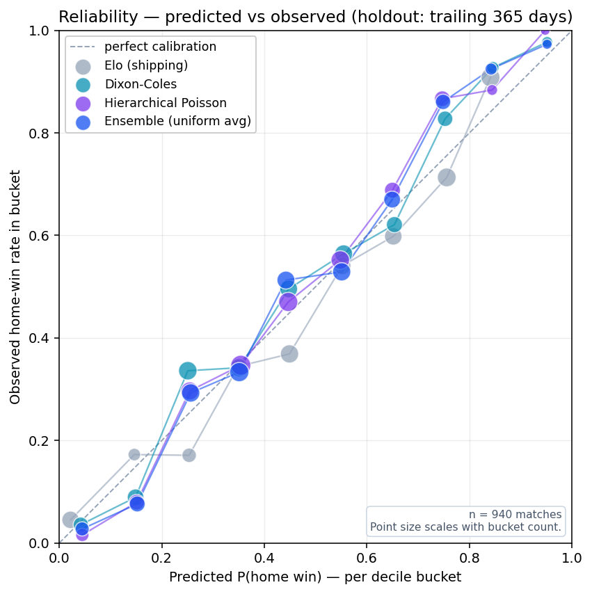
The plot above bins matches by predicted P(home win) into ten deciles and plots the observed home-win rate in each bin. A perfectly-calibrated model would lie on the dashed diagonal; points above the diagonal indicate the model is under-confident in the home team, points below indicate over-confidence.
Editorial scope
The project's editorial scope is bounded. The full constraints are documented in CLAUDE.md; the summary here is for context.
- The analytical universe is the model's own probabilities measured against ground-truth outcomes; published comparisons are model-vs-baseline (FIFA rank, observed frequency, historical analogues).
- Outputs are presented as probabilities and methodology — readers take them as research data and reach their own conclusions.
- The audience is researchers, journalists, fantasy players, analytics enthusiasts, and developers.
- Updates are batch — the pipeline refreshes on a daily cadence after results land, not in real time.
The scope is deliberate: these are publication choices, not constraints on what is statistically interesting.
Limitations and caveats
Honest disclosure of where the methodology is weak.
- Small sample of World-Cup-strength matches. International results since 1872 are plentiful, but matches between two top-thirty teams on neutral ground are concentrated in major-tournament knockouts and a handful of qualifying brackets, so the effective sample for the kind of fixture the 2026 tournament will produce is small.
- R32 is the published FIFA structure; R16 onwards is deterministic given group placings. The bracket structure is taken from the published 2026 format. Conditional on group outcomes, the knockout path is fixed — there is no draw randomisation past the group stage in our simulator. This reflects the format, not a modelling shortcut.
- International xG as the Poisson response — wired into production (2026-05-29). Replacing realised goals with
round(xG)was the roadmap's highest-leverage remaining lift. With the stale Opta mirror it never cleared the gate (~143 matches, ~3% coverage). Sourcing the gap from StatsBomb open data (single-provider, 342-match corpus — see "International xG as the response" above) cleared the gate for Dixon-Coles and the uniform Ensemble (tournaments-only ΔBrier_median −0.0023 / −0.0016, ECE improving). The auto-refit now fits DC with the xG response (HP excluded — its ECE drifts +0.21pp), with the ensemble calibrator refit on the xG-enabled ensemble; the xG-enabled artefacts regenerate on the first refit after the change lands. The residual limitation is StatsBomb open-data tournament coverage (Copa 2021 still Opta; qualifying cycles + friendlies remain on goals). - DC and Elo remain point estimates. Model 3 ships with a full Bayesian posterior; the other two component models do not. The credible interval published next to each tournament-stage probability propagates Model 3's posterior parameter uncertainty through the bracket Monte Carlo, but treats the Dixon-Coles MLE and the current Elo snapshot as fixed. A future version that adds posteriors on DC and on Elo would widen the bands further.
- Optimiser non-convergence flag (Model 2 only). Model 2's L-BFGS-B optimiser reports
converged=Falseeven though the predictions are stable and sensible at the reported parameters — the residual is in the sum-to-zero parameterisation rather than the fitted output. Model 3 (Hierarchical Poisson) now converges cleanly after a half-life andmaxfuntune. The Model 2 flag is cosmetic but worth disclosing. - Limited lineup awareness. Team strength is mostly carried by the per-team attack/defence parameters. The projected-XI composite differential (Model 16) and GK offset (Model 18) are both retired as no-ships after failing to clear noise thresholds (see respective sections above). Real-time lineup data for international football is operationally hard (no central archive, lineups arrive ~75 minutes before kickoff); lineup-derived adjustments remain a future research direction.
- Credible intervals reflect Model 3's posterior only. Per-team progression probabilities now carry a credible interval that propagates Model 3's PyMC NUTS posterior through the bracket Monte Carlo (1,000 posterior draws × ~5,000 inner MC sims per draw). Dixon-Coles and Elo are still fed in as point estimates, so the published band understates uncertainty by whatever those two components would contribute under their own posteriors. See "Uncertainty quantification" below.
- Backtest is now walk-forward, but eight folds is still a modest count. The eight-fold × 90-day walk-forward covers two years of international football; aggregating eight Brier numbers gives a more honest single-number summary than the previous single 365-day holdout, but it is not a substitute for a larger ablation set. Comparing two models that differ by ≲ 0.005 Brier still falls within the across-fold standard deviation; for changes that small, the per-fold + median view is what to read.
Uncertainty quantification
The published tournament-stage probabilities (p_advance, p_r16, p_qf, p_sf, p_final, tournament_prob) carry an optional confidence band, written to data/wc2026/bootstrap_intervals.json by scripts/bracket_mc.py --bootstrap. The band currently surfaces on the team card as a subscript next to the headline (17.3% [12.8%–22.4%] for the posterior regime, (12.8–22.4%) for the cheaper regimes) and inside the prediction-inputs popover.
Three regimes of band can be written, and they measure different things:
-
interval_kind = "posterior_uncertainty"(the canonical credible-interval regime). Each band point is a draw from Model 3's full Bayesian posterior (Hierarchical Poisson, fit by PyMC NUTS inscripts/fit_hierarchical_poisson_pymc.py) propagated through the bracket Monte Carlo. The 2.5th / 97.5th percentile across draws becomes the 95% credible interval. The band therefore reflects both posterior parameter uncertainty in the goal-scoring model and Monte Carlo sampling noise from the inner bracket simulator. Dixon-Coles and Elo are kept as point estimates inside the ensemble; widening the band to account for their uncertainty too is a follow-up. The CLI flag is--posterior-samples data/wc2026/hierarchical_poisson_samples.npz, and runtime is single-digit minutes at 100 draws × 2,000 inner sims. The.npzis produced once per refit cycle and re-used across snapshots. -
interval_kind = "parameter_bootstrap". Each band point is a separate refit of the Dixon-Coles + Hierarchical-Poisson ensemble on a bootstrap-resampled historical match dataset, run through the simulator at production sim count. This is a frequentist alternative to the posterior regime and is mainly retained as a sanity check on the Bayesian band. The canonical builder isbracket_mc.make_match_resample_snapshots(...); the CLI isscripts/bracket_mc.py --bootstrap --bootstrap-parameter --bootstrap-n 50 --bootstrap-sims 5000. Cost is ~3.5 hr at production sizes (~3-4 min per DC + HP refit × 50 snapshots, plus the bracket runs), so this regime is run offline on a separate cadence (not per-snapshot) — a monthlybootstrap-refitcron produces it. -
interval_kind = "sim_count_noise"(the cheapest legacy regime). The simulator is re-runn_bootstraptimes atsims_per_bootstrapMonte Carlo sims per run, with the same model parameters each time but different RNG seeds. The 5th and 95th percentile of those runs becomes the band. This captures Monte Carlo sampling noise at the reduced sim count, not parameter uncertainty. It is informative about how stable ansims_per_bootstrap-sim run is; it is not informative about how the published 100,000-sim point estimate compares to the "true" model output (sampling SE there is ~0.2pp at p = 0.5). Kept on disk as a fallback when the.npzis unavailable; the user-facing tooltip says explicitly that the band does not quantify parameter uncertainty.
The popover and team-card tooltip render copy that matches the actual interval_kind on file — posterior bands are labelled "Credible interval (Model 3 posterior)" and use square brackets in the subscript ([low–high]); parameter-bootstrap and sim-count bands are labelled honestly as what they actually measure.
Reproducibility
The pipeline is in scripts/. Each model has its own fitter and predictor:
scripts/bracket_mc.py— Model 1 (Elo + MC bracket, now consuming the calibrated ensemble for per-fixture probabilities).scripts/fit_dixon_coles.py— Model 2 fit.--use-xgswaps the per-match Poisson response from realised goals toround(xG)where available; the production auto-refit now runs this with--use-xg(see "International xG as the response").scripts/fit_hierarchical_poisson.py— Model 3 MAP fit, global-mean prior. Carries the--use-xgflag but is NOT on the production xG path — HP fails the gate's ECE half, so production fits HP on realised goals. Kept on disk as the gate-comparison baseline (seescripts/backtest_confed_hp_gate.py); no longer the production refit path.scripts/fit_hierarchical_poisson_confed.py— Model 3b MAP fit, confederation-pool prior. Same output JSON schema as the global-mean variant (drop-in forensemble.py/bracket_mc). This is the script the auto-refit workflows call per the §16 gate (see "Model 3b" above). Realised goals only (not on the xG path).scripts/pull_intl_xg.py— Legacy Opta puller: per-match xG from the FBref / JaseZiv mirror intodata/raw/intl/xg.csv(~143 matches, now stale). Superseded for production by the StatsBomb puller below; retained for the 28 Copa-2021 rows StatsBomb lacks.scripts/pull_intl_xg_statsbomb.py— Production xG puller. Per-match team xG (Σshot.statsbomb_xg) from StatsBomb open data for WC 2018/2022, Euro 2020/2024, Copa 2024, AFCON 2023;--merge-intounions with the residual Opta Copa-2021 rows (StatsBomb-preferred, orientation-aware) into the single-provider 342-rowdata/raw/intl/xg.csv. See "International xG as the response" above.scripts/fit_hierarchical_poisson_pymc.py— Model 3 full posterior via PyMC NUTS (1,000 warmup + 1,000 sampling × 4 chains; R-hat ≤ 1.01, ESS ≥ 400 gated). Writes the posterior.npzconsumed by the bracket Monte Carlo to produce credible intervals.scripts/ensemble.py— uniform-average combiner; applies the isotonic calibrator at predict-time.scripts/fit_ensemble_calibrator.py— fits the per-class isotonic curves and writesdata/wc2026/ensemble_calibrator.json.scripts/isotonic.py— pure-Python pool-adjacent-violators implementation used by the calibrator.scripts/build_ratings_player.py— splices per-player season stats intodata/wc2026/ratings_player.csv.scripts/build_player_composite.py— Model 4 (per-player [0, 1] composite rating).scripts/build_gk_rating.py— Model 4b (goalkeeper-specific rating).scripts/build_anytime_scorer.py— Model 5 (tournament-scorer probability).scripts/pk_proficiency.py— Model 15 (PK shootout proficiency).scripts/historical_analogues.py,scripts/counterfactuals.py,scripts/counter_narrative.py— Tier-A explainability and editorial-novelty layer.scripts/backtest_models.py— produces the comparative numbers above.
Data sources are pulled by scripts/pull_*.py. The pipeline is documented in more depth in documentation/data-sources.md, documentation/team-modeling.md, and documentation/player-quality.md.
Versioning and updates
This page describes the methodology as of the 2026 tournament cycle. Material changes (new model, new data source, calibration retraining) will be noted in the project changelog. The page is intended to remain accurate as the methodology evolves; any future divergence between this page and the deployed pipeline is a bug.